how to add legend in excel
The key to understanding charts is through the use of legends. Legends are automatically created everytime we create a graph or plot our data.
 Figure 1. Final result: How to edit legend
In the chart above, the legend is located in the top center of the graph, showing a bulleted list with text "A" and "B Sales".
When we encounter an Excel chart without a legend, we can easily add a legend through these steps:
Add legend to an Excel chart
Step 1. Click anywhere on the chart
Step 2. Click the Layout tab, then Legend
Step 3. From the Legend drop-down menu, select the position we prefer for the legend
Example: Select Show Legend at Right
 Figure 2. Adding a legend
The legend will then appear in the right side of the graph.
 Figure 3. Output: Add legend to a chart
The legend in a chart can be edited by changing the name, or customizing its position and format.
How to change legend name?
There are two ways to change the legend name:
- Change series name in Select Data
- Change legend name
Change Series Name in Select Data
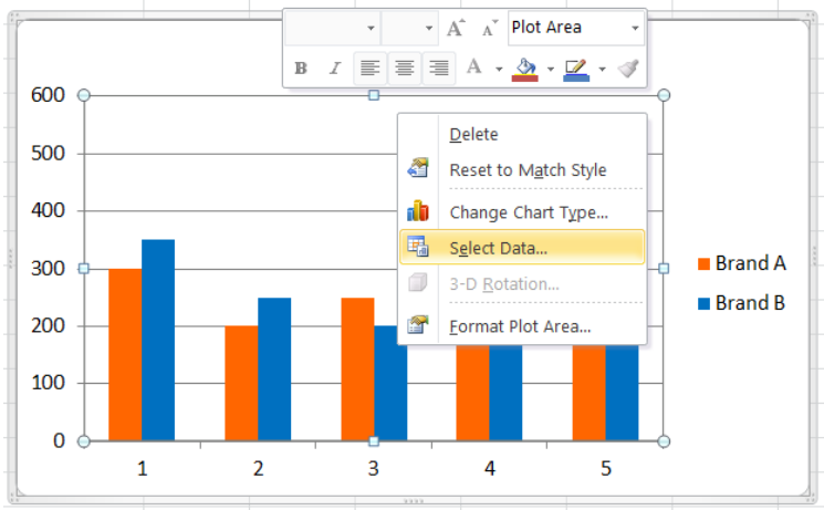
Step 1. Right-click anywhere on the chart and click Select Data
 Figure 4. Change legend text through Select Data
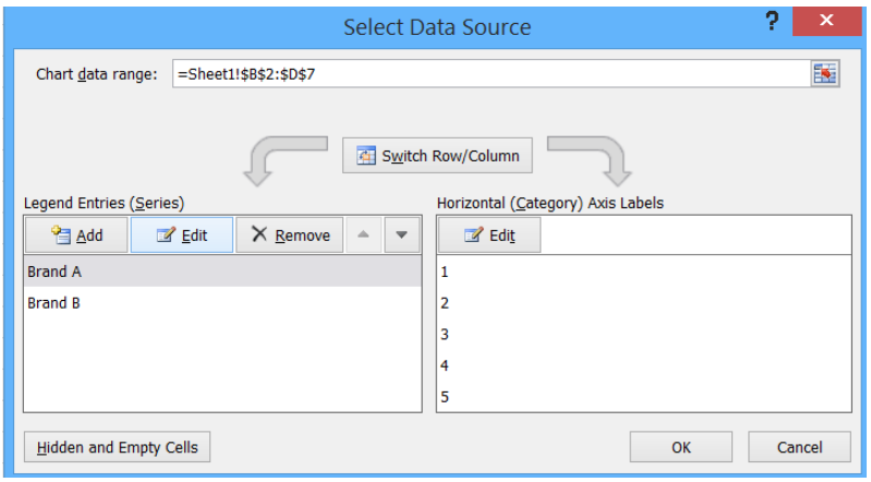
Step 2. Select the series Brand A and click Edit
 Figure 5. Edit Series in Excel
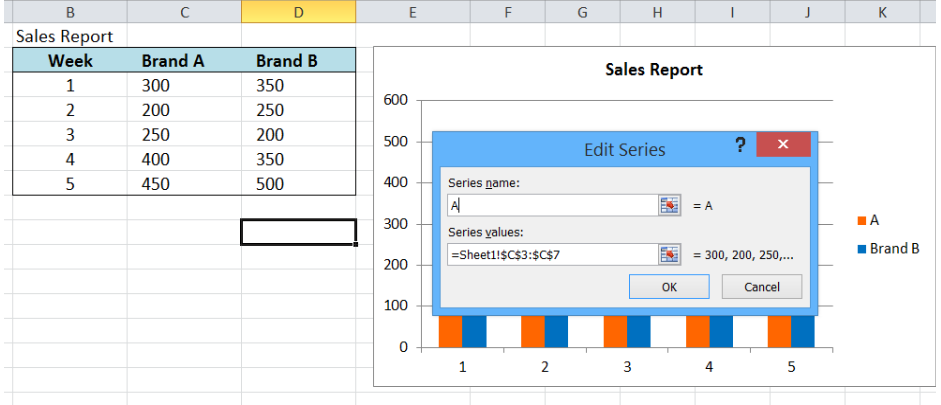
The Edit Series dialog box will pop-up.
 Figure 6. Edit Series preview pane
Step 3. Delete the current entry "=Sheet1!$C$2" in series name and enter " A " into the text box.
 Figure 7. Changing legend text
The legend name is immediately changed to "A".
 Figure 8. Output: How to rename legend
Change legend name
Step 1. First, we must determine the cell that contains the legend name for our chart by clicking the chart. As shown below, the column chart for Brand B is linked to cells D2:D7 .
 Figure 9. Change legend text
Step 2. Since D2 contains the legend name, we select D2 and type the new legend name "B Sales".
 Figure 10. Change legend name
As shown above, the legend name on the chart is instantly updated from " Brand B " to " B Sales ".
How to edit legend?
Legends can be customized by changing the layout, position or format.
How to change legend position?
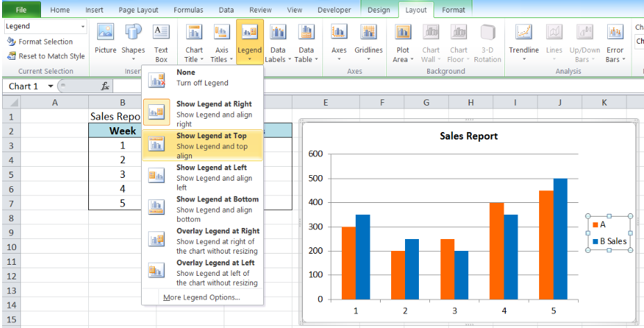
It is very easy to change the legend position in Excel. Simply click the chart, then click the Layout tab. Under Legend , choose the preferred position from the drop-down menu.
 Figure 11. Change legend position
Example :
Select Show Legend at Top from the drop-down menu. As shown below, the legend is transferred to the top of the chart.
 Figure 12. Output: Change legend position
How to edit legend format?
In order to change the format, right-click the legend and select Format Legend .
 Figure 13. Edit legend through Format Legend
The Format Legend dialog box will appear. There are several options where we can change the legend position, fill, border color, border styles, and other formatting options.
 Figure 14. Format legend preview pane
Example :
We want to fill the legend box with Aqua, Accent 5, Lighter 60%.
We click Fill , then tick Solid Fill .
 Figure 15. Change legend fill
Choose the color we prefer and click OK. The fill color will automatically be updated to the chosen color.
 Figure 16. Select fill color for legend
We can add more formatting changes. Below chart shows the legend format with a 5% pattern fill and an orange border color.
 Figure 17. Final result: How to edit legend
Instant Connection to an Expert through our Excelchat Service
Most of the time, the problem you will need to solve will be more complex than a simple application of a formula or function. If you want to save hours of research and frustration, try our live Excelchat service! Our Excel Experts are available 24/7 to answer any Excel question you may have. We guarantee a connection within 30 seconds and a customized solution within 20 minutes.
how to add legend in excel
Source: https://www.got-it.ai/solutions/excel-chat/excel-tutorial/legend/how-to-edit-legend-in-excel
Posted by: klattmort1951.blogspot.com

0 Response to "how to add legend in excel"
Post a Comment